The following will act as lecture notes to help you review the material from lecture for the
assignment. You can click on the links below to get directed to the appropriate section or
subsection.
One common application of computer graphics animation is the simulation of physical systems
such as the swinging of a simple pendulum or the flow of air over an airfoil. In these simulations,
we want to graphically model the behavior of natural phenomena as they evolve dynamically in
time. In order to model the behaviors correctly, we not only need to focus on the graphics that we
display but also on the numerical computations that determine the state of a physical system at a
particular point in time.
A state of a physical system refers to the conditions that define the system at a
particular point in time. For instance, consider a ball bouncing vertically in a frictionless
environment. At any given moment in time, we can specify the state of the system
with the height of the ball relative to the ground and the vertical velocity of the ball.
This essentially gives us a snapshot of the configuration of the system at some time
.
The evolution of a system from the state at time
to the
state at time
is often governed by a system of differential equations that is generally hard or impossible to solve
analytically. In many cases, we must resort to using numerical methods to approximate the
changes in conditions between states, starting with the initial conditions for the initial state of the
system. We refer to these numerical methods specifically as time integration techniques or timeintegrators.
As an example of a time integrator, recall Euler’s method from introductory calculus: given a position
and velocity
at time
and an acceleration
function , we compute
the conditions for time
using the equations:
In addition to Euler’s method, there are many other time integrators out there, though
not all of them are equal in being “reliable” for graphical simulations. In the following
subsections, we discuss one particularly appropriate family of integrators for computer
graphics known as variational time integrators, which are derived from Lagrangianmechanics.
We start off by first examining a simple example of a physical system to demonstrate the
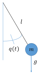
different behaviors of different time integrators. Consider a simple pendulum of mass
and
length ,
swinging in a frictionless medium under the influence of the gravitational acceleration
.
The pendulum only has one degree of freedom in its angle, which we will denote
. Figure
1 shows a visual of the system:
Figure 1: A simple pendulum with mass
and length
moving in a frictionless environment under the influence of gravity. We denote the angle at
a given time
as
.
We know from simple physics that the equation of motion for this system is given by:
where we use the dot notation to denote derivatives with respect to time.
From here, we could theoretically solve for an analytical solution to the system if we
were to make a small angle approximation. However, for the sake of the example, let us
assume that an analytical solution is not possible (as is the case for many other systems).
We would then need to approximate the time evolution of the system using a time
integrator.
Let us first try to model the system using the Euler’s method we used in introductory calculus. We
will refer to this method by its more technical name: the explicit Euler method. It is also often
called the forward Euler method.
The explicit Euler method is often taught in introductory calculus classes as simply
“Euler’s method.” For our convenience, we will reiterate the method here: given a position
and velocity
at time
and an acceleration
function , we compute
the conditions for time
using the update rules:
To apply the explicit Euler method to the simple pendulum system, we first need to discretize the
problem and introduce some notation. We break up the time between our initial time
and our final time
of simulation into
equal time steps of
length . We denote
the time at the -th
time step as for
. The angle of the
pendulum at time
is denoted as .
Let so that
is the angular velocity of
the pendulum at time .
Using the above notation, we write the explicit Euler update rules as so:
These equations are referred to as explicit equations. Given the values
and
at time
step ,
we can use the above update rules to explicitly compute the values
and
at the next
time step .
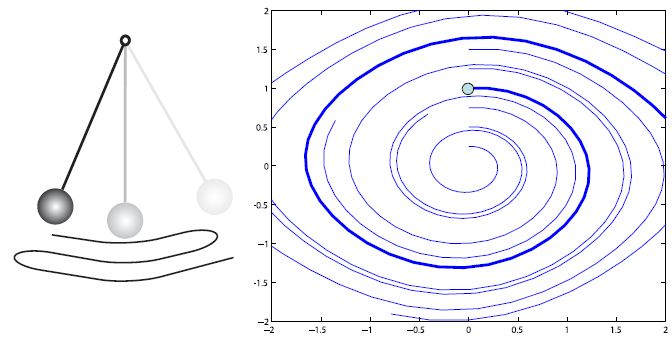
Let us now examine the performance of this integrator. Consider Figure 2:
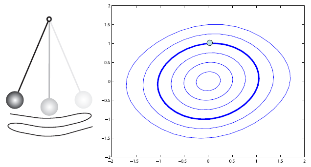
Figure 2: A visual of the behavior of the explicit Euler integrator. On the left, we see that
the amplitude of the pendulum increases as the pendulum continues to swing. On the right
is a phase portrait of the system with the angle
on the x-axis and the angular velocity
on the y-axis. The dot marks the initial point corresponding to the initial values of
and
.
We see from the phase portrait that the values of
and
continuously increase and “spiral outwards” from the initial point. This diagram is taken
from [1].
Figure 2 shows a visual display of the behavior of the explicit Euler integrator. On the left is a
display of how the amplitude of the pendulum changes as time goes on. We see that the explicit
Euler integrator actually causes the amplitude to increase with passing time. The phase portrait on
the right conveys this information in a different manner. Here, we see that the angle
, represented by the
x-axis, and velocity ,
represented by the y-axis, both continuously increase from their initial values, which we mark with
the dot. The outward “spiral” shown in the phase potrait tells us that the pendulum will move
further and faster as time goes on, suggesting a numerical instability where the energy of the
system “blows up” and goes towards infinity.
This “blowing up” behavior modeled by the explicit Euler integrator is obviously incorrect. In
reality, the energy of the simple pendulum system is conserved, and the amplitude of the pendulum
should remain constant. The explicit Euler integrator therefore is not a reliableintegrator for simulating physical systems.
What causes this ”blowing up” behavior? To answer this question, we can examine
what exactly goes on in the update rules of the explicit Euler integrator. Both the
update rules for the integrator are actually first order Taylor approximations. Given
and
, we compute
and
using the tangentslopes of and
respectively
at time .
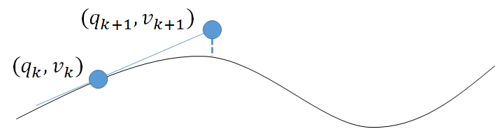
Figure 3 demonstrates this with a visual:
Figure 3: The explicit Euler integrator makes first order Taylor approximations. Given
and
,
we use the slopes of the tangents at time step
to compute
and
.
The nature of this approximation causes the integrator to accumulate error at each time
step, leading to numerical instability.
Let the curve in Figure 3 represent the path of motion of the system in
phase space. We then see that using a first order Taylor approximation for
and
leads us to a
point that is off the actual path of the system. Because this point is off, the subsequent approximation
for
and ,
which depends on the tangent at this “off” point, would then lead to another point that is even
further off from the actual path of the system. As we continue making these approximations, the
error between the approximated values and the true values will accumulate, eventually causing the
approximated values to approach infinity. This results in the “blow up” behavior we see in Figure
2.
Knowing that the explicit Euler method is unreliable, let us try out a different time integrator:
the implicit Euler method. This method is also often called the backward Eulermethod.
The implicit Euler method is another popular time integrator that is a counterpart to the
explicit Euler method. The implicit Euler method takes the update rules of the explicit Euler
method and evaluates their right hand sides at the next time step. This causes the update rules to
take the form of a set of non-linear equations.
Using the same notation as before, we write the implicit Euler update rules for the simple
pendulum system as so:
These equations are referred to as implicit equations as opposed to
explicit equations and require the use of a non-linear solver to compute
and
given
and
. We
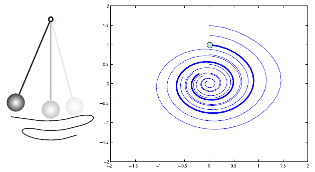
examine the behavior of implicit Euler in Figure 4:
Figure 4: A visual of the behavior of the implicit Euler integrator. On the left, we see that
the amplitude of the pendulum decreases as the pendulum continues to swing. On the right
is a phase portrait of the system with the angle
on the x-axis and the angular velocity
on the y-axis. The dot marks the initial point corresponding to the initial values of
and
.
We see from the phase portrait that the values of
and
continuously decrease and “spiral inwards” from the initial point. This diagram is taken
from [1].
Figure 4 shows the behavior of the implicit Euler integrator similar to how Figure 2 shows the
behavior of the explicit Euler integrator. We see on the left that the implicit Euler integrator
causes the amplitude of the pendulum to decrease with passing time. The phase portrait tells us
that
and
both continuously decrease from their initial values, forming an inward “spiral” that suggests
numerical dissipation. That is, the energy of the system is artificially dampened by the
integrator and goes towards 0.
While the implicit Euler method is not numerically unstable like the explicit Euler method, it
also does not correctly conserve the energy of the system. This is not too surprising,
since the implicit Euler method is essentially a reverse explicit Euler (hence the name
“backward Euler”). We can see this by rearranging the update rules for implicit Euler as
so:
The above equations show that the implicit Euler is just explicit Euler going backwards in time.
Thus, implicit Euler also suffers from error due to first order approximations and isnot a reliable integrator for simulating physical systems.
What integrator should we use then if both explicit and implicit integrators are unsatisfactory?
There is an integrator known as the symplectic Euler method or semi-implicit Eulermethod, which involves a “strange mix” of the explicit and implicit update rules. The update
rules as applied to the simple pendulum system are:
The idea here is to first explicitly compute
and then implicitly use
to compute .
The results of this integrator are shown in Figure 5:
Figure 5: A visual of the behavior of the symplectic Euler integrator. On the left, we see
that the amplitude of the pendulum remains constant as the pendulum continues to swing.
On the right is a phase portrait of the system with the angle
on the x-axis and the angular velocity
on the y-axis. The dot marks the initial point corresponding to the initial values of
and
.
We see from the phase portrait that the values of
and
are conserved. This diagram is taken from [1].
Similar to Figures 2 and 4, Figure 5 shows the behavior of the symplectic Euler integrator. We see
from both the pendulum diagram and the phase portrait that the symplectic Euler methoddoes correctly conserve the energy of the system.
The question now is why. Why does the symplectic Euler method produce reliable results? Also,
how would we have come up with this “strange mix” of an integrator?
We will find in the following sections that the reason the symplectic Euler method correctly
conserves the energy of a system is because it is derived from a principle from Lagrangianmechanics that takes into account the entire path (i.e. all the states) that the system takes to go
from its initial state to its final state. In comparison, neither the forward nor implicit Euler
methods consider the entire path of the system; instead, they both only consider the time evolution
of the system one state at a time.
We present, in this section, a brief overview of Lagrangian mechanics as necessary for the
understanding of creating reliable time integrators. Do note though that, because this class is not a
physics class, our overview is not very rigorous. For those students who are interested in
learning Lagrangian mechanics in depth, we recommend taking an advanced classical
mechanics course. Additionally, [2] also provides a rigorous, in-depth analysis of what
we cover in the following sections and more (although the work does contain a few
typos).
At the root of Lagrangian mechanics lies the Lagrangian, which is defined to be the difference
between the kinetic and potential energies of a physical system:
where denotes the
Lagrangian, denotes
kinetic energy, and
denotes potential energy.
and
denote our position and velocity state vectors respectively.
We define what is called the action, denoted by
,
as:
To get an intuitive understanding of what the action is, let us examine for
a moment the simple physical system involving a ball thrown from position
to position
.
Physics causes the ball to take a certain trajectory or path
as it moves
from
to . We
can compute the Lagrangian for each point along this path, and the sum of all the computed
Lagrangian values gives us the action.
The reason why we introduce this concept of “action” is because of a key principle in physics
known as Hamilton’s least action principle, which states that the action of a physical system
is always at a extremum (e.g. minimum). Now, before we discuss what it means for the action to
be at an extremum, let us step back and consider what it means for a simple function
to be extremized
at a point . For
to be a extremum,
we know that .
From this, we might be tempted to say that for the action,
,
to be at a extremum, the derivative of the action with respect to
must be 0. The issue with
this statement is that, unlike ,
does
not just represent a single value. Rather, because the action is defined to be an integral over the
values
to ,
is actually
a path
between the initial and final states. This makes examining the extremum of the action a bit more
complicated than what we are used to.
The key to understanding the impact of the least action principle lies in what we call variationalcalculus. Of course, an overview of variational calculus is beyond the scope of this course. For our
purposes, we simply need to know that the analog of the derivative that we need for
examining the extremum of the action is known as the variation, which we denote with
. Conceptually, a
variation of a path ,
denoted as ,
is an infinitesimal perturbation (i.e. deviation) to the path at each point
except at the endpoints, where the perturbations are null. Similar to how
when
is a
extremum,
when
is a extremum.
We compute the variation of the action as so:
Using integration by parts yields:
Now, because the perturbations at the endpoints of
have to be null,
we have that .
This causes the rightmost term of the right-hand side to vanish. Following the least action principle, we
then set
and obtain:
From here, we invoke what is called the fundamental lemma of calculus of
variations, which tells us that, because the above integral equals 0 for all
, the
part of the integrand in the square brackets also equals 0. Applying this lemma gives us the
following important formula:
The above formula is known as the Euler-Lagrange equation and is essentially the core of
Lagrangian mechanics. For a given Lagrangian of a physical system, we can use the Euler-Lagrange
equations to derive the equations of motion of the system.
As a demonstration of the power of the Euler-Lagrange equations, consider a physical system involving a particle of mass
moving under the influence
of a potential function ,
where we use
to denote the position of the particle. The Lagrangian of the system is simply:
Plugging
into the Euler-Lagrange equations yields:
which we can express as:
And we see that we obtain Netwon’s law of ,
which is what we would expect as the equation of motion for this system.
So what about Lagrangian mechanics allows us to create reliable integrators? The answer to this
question lies in the fact that the action is a function of the entire path that the given system
takes from its initial state to its final state. This fact causes the action to encode the
global behavior (i.e. behavior throughout all of time) of the system. And because the
Euler-Lagrange equations are derived directly from the action, they inherently also
encode the global behavior of the system. As a result, any equations of motion derived
from the Euler-Lagrange equations would also inherently take into account the global
behavior.
Now, let us say that we manage to construct a complete, discrete equivalent of the action that –
like its continuous counterpart – encodes the global behavior of the given system. The updaterules that we derive from this discrete action would then also inherently take intoaccount the global behavior. The following subsection details how we construct
this discrete action and subsequently derive from it the discrete Euler-Lagrangeequations.
Let us first consider how we compute integrals in the discrete setting in general. Given an integral of a
function
from
to , we can
approximate the integral by summing up rectangle approximations of the area under the curve formed by
at discrete time
steps of length .
Let
be the number of time steps. The area of the rectangle at time step
for
is given by
. The
overall integral is then computed via:
We use the same thought process as above to construct a discrete equivalent
of the action. We first define the discrete Lagrangian, denoted by
, as the
area of a discrete rectangle given by:
where denotes
the continuous Lagrangian of the system of interest. Note that we use above a discrete approximation of
, which, for a discrete time
step, can be written as .
Hence, the discrete Lagrangian ends up being a function of two consecutive states,
and
, and the size of
the time step, .
We then write the discrete action as:
Following the continuous derivation of the Euler-Lagrange equations, we express the variation of
the discrete action as:
where we use to denote the
derivative of with respect
to the first argument, ,
and to denote the
derivative of with respect
to the second argument, .
We can rearrange the sum of
to obtain:
Remember that we require the variations at the boundary points,
and
, to be
0. This eliminates the two terms outside the summation. From here, we follow the continuous
derivation of the Euler-Lagrange equations and set the variation of the discrete action to
0:
Because the sum is 0 for all ,
the expression within the sum must be 0. Hence, we obtain:
(1)
We refer to the above as the discrete Euler-Lagrange (DEL) equations. Given two consecutive
states (i.e.
and ),
we can use the discrete Euler-Lagrange equations to solve for the next state (i.e.
).
We can, however, go further and derive a more useful form of the DEL equations. To do so, let us
first consider the DEL equations for the simple Lagrangian:
The discrete Lagrangian for this system is:
Observe what happens when we compute:
Note how the right-hand side of the equation is just the momentum at time step
, which we will
denote . It turns out
that, in general,
is indeed just
for any Lagrangian. The full proof of this is outside the scope of this class, but we can at least see
from the above example how this can be true.
Now, from the above fact and the DEL equations, we have:
The above means that we can write the DEL equations in the following form:
(2)
(3)
Consider for a moment the power of the above two equations. Giventhe position and momentum of a physical system at some state, wecan solve the above two equations for the position and momentum of the next state.
Unlike the previous form of the DEL equations, which required two consecutive states to compute
the next state, this form only needs one state (i.e. the state at the current time step) to compute
the next state.
Equations (2) and (3) are the main DEL equations and are what we use to createreliable time integrators. Because they were derived from the action, which takes into
account the entire path of the given system, the DEL equations and any time integrators
derived from them inherently account for the global behavior of the system. We refer
to the time integrators that we derive from the DEL equations as variational timeintegrators.
To demonstate the power of the DEL equations, we will derive the sympletic Euler integrator for
the simple pendulum system that we analyzed earlier.
We start by writing the continuous Lagrangian for the system:
Using the relationships:
we can rewrite the Lagrangian in terms of
and
as:
The discrete Lagrangian is then:
Computing the respective derivatives gives us:
Now, recall from classical mechanics that the angular momentum of a simple pendulum is
, where
is the angular velocity.
Substituting this definition of
into the above equations and doing some algebra simplifies the above two equations into the
following equations:
A little rearranging and substitution finally gives us:
which are exactly the equations that we introduced previously as the symplectic Euler
integrator!
When we animate scenes in computer graphics, we often use a technique called keyframeinterpolation to generate the animation. The idea of keyframe interpolation is best introduced
with an example, so let us consider the following scenario.
We want to create a minute-long, traditional animation where each frame is hand-drawn. For the
animation to appear smooth, we need to display around 30 frames per second. However, 30 frames
per second for 60 seconds results in a grand total of 1800 frames to be drawn! And that is only for
a minute-long animation. The amount of time and manpower it would take to generate all the
frames necessary for an even longer animation would be enormous. However, with the advent of
computer animation, we can now generate long animations by drawing only a small
number of select frames called keyframes. We draw the keyframes, which capture the
most important scenes in our animation, and generate the rest of the animation by
interpolating or, in other words, using computer algorithms to “fill in the gaps” between the
keyframes.
One particular way of specifying a keyframe is with the positions and orientations of all the
points in the scene of interest. We specify the position of a point as a translation from an arbitrary
chosen origin and the orientation of a point as a rotation by an angle about some axis. In addition,
we also find it convenient to specify the scaling of a point as another characterization of the point’s
configuration in a scene. When we interpolate between keyframes, we actually interpolate
the change in translation, rotation, and scaling of each point in the scene between the
frames.
We most often interpolate across keyframes by piecing together individual polynomial curves to
form an overall, piecewise polynomial function called a spline. The spline goes through
and connects all corresponding points across all keyframes. To see how this process
works, let us consider piecing together a spline based on linear interpolation between
keyframes.
Let us say that we currently have two keyframes,
and
, that we want to linearly
interpolate between. In ,
we have a point that is positioned in the scene by the translation vector
. In
,
that same point is now positioned in the scene by the translation vector
. The scenes
in both keyframes use the same coordinate system. To linearly interpolate the change in position of the
point between
and ,
we need to linearly interpolate between the translations vectors
and
.
Our linear interpolation scheme proceeds as follows. First, we should note that
we need to interpolate the components of the translation vectors oneat a time. However, for simplicity in the notation, we will still use the variables,
and
, to
denote the values that we are interpolating. Now, consider a line segment connecting
to
. We
parameterize this line segment over the unit domain with the following function:
where . We can then
use to compute
the values between
and to
“fill in” the motion that our point takes as it moves between the two keyframes.
Now, for reasons that we will see later, we find it convenient to consider the following alternative
formulation of :
for coefficients
and .
We notice that the above formulation is the canonical representation of a first degree
polynomial (i.e. a line). We can rewrite this formulation using vector notation. Let
and
. Then,
we have:
What exactly is though?
Well, we know that
and . We also
know that for ,
we have .
And for ,
we have .
With this, we can write the following system of equations:
Let us write the above system as:
where we call
the constraint matrix. Note how we can solve for
after finding the
inverse of . We denote
the inverse of
with the variable
and call it the basis matrix. We can now evaluate the curve between
and
as:
We repeat the above process for each pair of values
and
in consecutive
keyframes
and . In
the end, we obtain multiple line segments that connect sequentially to form a spline that goes through
all points .
We can use the pieces of the spline to compute the components of all translation vectors needed
between keyframes to generate the animation across all keyframes.
Now, at this point, one might ask, “why did we have to make this process so complicated?” After
all, our original, parameteric formulation would have been sufficient for the interpolation between
two points. The answer is that while this process is unnecessary for simple linear interpolation, the
whole concept of computing constraint and basis matrices becomes useful when we interpolate
using more complicated curves.
Furthermore, we can imagine that simply using linear interpolation between keyframes would not
produce smooth motion. Consider the shape of a spline formed from only line segments.
Line segments do not transition smoothly into one another; rather, they form sharp
angles at each junction. These sharp angles cause the motion of the point to result in
sudden changes as we transition between keyframes. As a result, we do not obtain smooth
motion from linear splines and must instead look towards more complicated curves for
interpolation.
Before we continue, let us stop to consider the nature of a spline that would produce smooth
interpolation across keyframes. We know that a spline consisting of line segments does not work
because the segments form sharp angles at each junction. What is a condition that we can enforce
to prevent our spline from having sharp angles?
The answer is to require the first derivatives of two connecting pieces of our spline to be equal at the
junction (i.e.
continuity). This means that we must, at the very least, use quadratics for interpolation.
It turns out that cubics are the most commonly used polynomials for keyframe interpolation. In
particular, we often use a specific class of cubics called cardinal cubic curves. We
call the overall resulting curve a cardinal spline. They have the nice properties of
and
continuity (i.e. their first and second derivatives are continuous everywhere).
We form a cardinal cubic curve in the following manner. First, let us denote the two keyframes that we are
interpolating between as
and .
Let
and be
the values (e.g. components of translation or scaling vectors) that we are interpolating between the
two keyframes. To form a cardinal cubic curve, we need to also consider the keyframes,
and
and their
corresponding values,
and .
Thus, the cardinal cubic curve has four control points indexed from
to
.
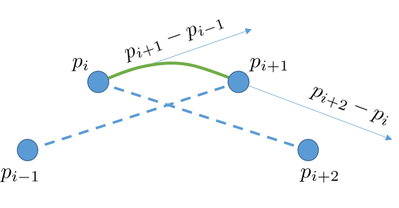
We let the derivative at the beginning of our curve segment be a scaling of the vector between the
first and third control points. And we let the derivative at the end of our curve segment be a
scaling of the vector between the second and fourth control points. Figure 1 below provides a visual
of this.
Figure 1: A visual of the formation of a cardinal curve (in green) used to interpolate
between
to
.
Four control points are necessary. The derivative at the beginning of the curve is a scaling
of the vector between the first and third control points. The derivative at the end of the
curve is a scaling of the vector between the second and fourth control points.
Let us take a moment to convince ourselves that the derivatives of two consecutive
cardinal curves match at the point in which the curves connect. Consider a cardinal curve
between
points and
connecting to a
cardinal curve
between points and
. The two curves
connect at point .
Now, the derivative of
at is given
by -
,
the difference between the second and fourth control points of
. What is the
derivative of
at ?
It would the the difference between the first and third control points of
. The first and third
control points would be
and respectively,
hence, the derivative of
at would
also be -
. Thus, the derivatives
match at point .
Similar logic can be used to confirm that the derivatives at other junctions along a cardinal spline
also match.
To find a mathematical representation for the cardinal curve, we undergo a process similar to the one
we took for our linear interpolation example above. We first represent the cardinal curve between
and
with a
function, ,
that is parameterized over the unit domain. Our constraints for the curve then can be expressed
as:
where
is the scaling factor for the derivative vectors. We formally define
to
be:
where is known
as the tension parameter and is an arbitrarily set value that controls the bending of the curve. The
closer we set
to 1, the flatter the curve becomes around the control points. We often, however, simply set
to 0. We call the
set of splines for
Catmull-Rom splines.
Since cardinal curves are cubics, we will consider the canonical representation of a third degree
polynomial:
for
and .
We want to now write a system of equations in the form of
. To do
so, we consider our constraints and solve for the control points:
Substituting our canonical cubic polynomial into the above set of equations yields:
which we can express in the form of .
Taking the inverse of the resulting constraint matrix yields the following basis matrix:
For the case where
(i.e. for Catmull-Rom splines), we have:
Hence, our cardinal curve function can be expressed as:
Given four control points expressed as and an appropriate parameter, we can use the above to compute the interpolated values betweenand. This
interpolation method smoothly interpolates the components of both translation and scaling
vectors.
To interpolate the rotation quaternions, simply use this interpolation method on each
component of the keyframe rotation quaternions, then normalize the result. Refer back to our
Assignment 3 lecture notes for details about quaternions.
There are other methods for rotation interpolation, including Spherical Linear Interpolation (SLERP)
[3] [4], which interpolates quaternions along the great arc of a sphere. However, SLERP does not
have
or
continuity because it only uses the nearest two control points for interpolation. Thus, it can
produce awkward motion in comparison to more sophisticated methods [5].
Another major class of splines is the B-spline, which is a type of non-interpolating spline. This
means that a B-spline is not required to pass through its control points. An extension of
B-splines called NURBS (Nonuniform rational B-splines) can have control points that are
non-uniformly spaced apart. This is useful for adding control points to a NURBS
curve without affecting the shape of the curve, which is extremely useful in modeling for
allowing more local control of the curve. NURBS can also be used to define smoothsurfaces in 3D using a technique called lofting, which combine two NURBS curves into a
single surface. If you are interested in reading about the details behind NURBS and
B-splines in general, feel free to check out these notes on NURBS and NURBS surfaces
from previous years of CS171. For an interactive website which allows you to see how
B-splines and NURBS splines change when you move the control points, click here and
here.